Algorithmic repricing raises prices only where rivals also automate
An example seminar deck, generated end to end with Claude Code
Claude Code
September 18, 2026
Most prices on this marketplace are now set by software
- 68% of active listings change price at least once a week, against 4% in 2015.
- Repricing is delegated to a handful of third-party tools whose rules are published.
- Sellers meet the same rivals week after week, so rules respond to rules.
The policy question is usually posed as whether automation is inflationary. That framing is incomplete: the answer depends on the composition of the market a seller automates into.
Source: PriceScope weekly listing panel, 2015–2023. Own calculations. Online price competition on this kind of marketplace has been measured since Chevalier and Goolsbee (2003).
Automation pulls prices in two directions at once
Delegating price setting cuts the cost of a revision from roughly $14 of seller attention to near zero. Two consequences run in opposite directions.
- Cheap revisions let a seller undercut a slow rival within hours, which pushes prices down toward marginal cost.
- Cheap revisions also make undercutting visible and matchable within hours, which sustains higher prices when rivals are equally fast.
Which force dominates is a question about the rival mix \(\mathrm{RivalShare}_{mt}\), the share of a market’s listings already under automated pricing, not about automation itself.
Both forces are old; what is new is that they can now run at machine speed. Undercutting is the mechanism Chevalier and Goolsbee (2003) find between two online booksellers, and the variety it is traded against is what Brynjolfsson et al. (2003) price (see also Chevalier and Mayzlin 2006).
Automation raises prices only where rivals automate too
Headline estimate Adoption raises a listing’s price by 6.2 log points (s.e. 1.4) in the top quartile of rival exposure, and by −0.4 (1.1) in the bottom quartile.
The two estimates come from the same regression, the same sellers, and the same weeks. The sign of the effect of automation is a property of the market, not of the technology.
Automation is not inflationary on its own. It is inflationary where it is already common.
Setting and identification
API access arrived in a queue, not by application
- 41,208 listings across 320 narrow product markets, priced weekly, 2015–2023.
- API access arrived by seller tier between March 2019 and November 2021, with no application and no way to move up the queue.
- A listing is coded as automated in the first week its price changes on three or more distinct days, a threshold no manual seller in the pre-period ever crosses.
Rival exposure \(\mathrm{RivalShare}_{mt}\) is the share of other listings in market \(m\) and week \(t\) coded as automated.
A queue rollout is a design used elsewhere: Wiles et al. (2025) identify the effect of algorithmic writing assistance the same way, on hires rather than prices.
Adoption tracks the tier queue that granted API access
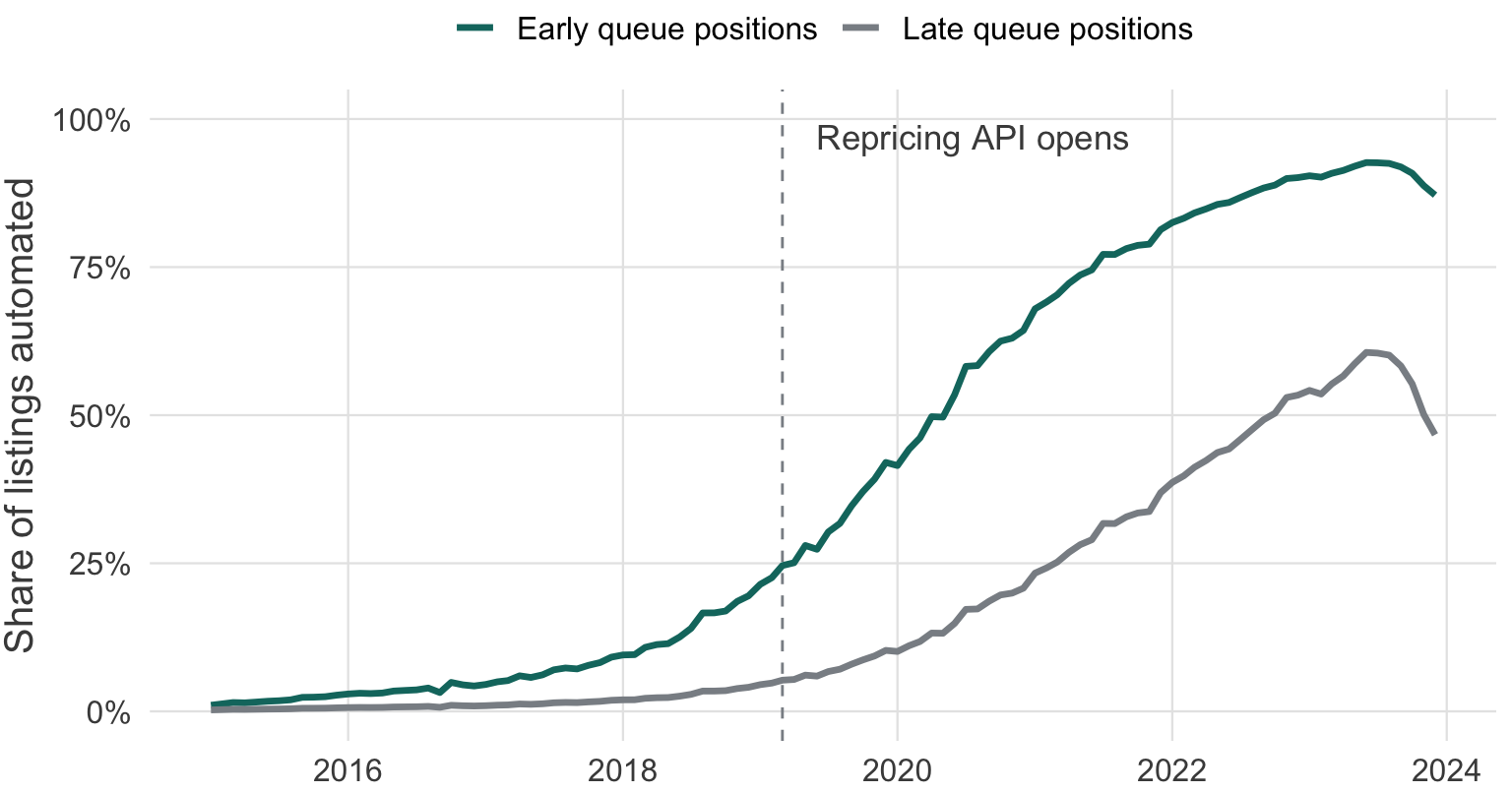
Figure 1: Adoption of the repricing API, by queue position
Groups are the earliest and latest thirds of the queue, fixed at seller signup. Seller behaviour on this marketplace has mostly been studied through reviews rather than prices (He et al. 2022).
Identification compares adopters to not-yet-adopters inside the same market-week
\[ \begin{aligned} \log p_{jmt} = \;& \beta_1 A_{jt} + \beta_2 \bigl(A_{jt} \times \mathrm{RivalShare}_{mt}\bigr) \\[2pt] & + \gamma_j + \delta_{mt} + \varepsilon_{jmt} \end{aligned} \]
Here \(A_{jt} \in \{0,1\}\) marks automation, \(\gamma_j\) absorbs the listing and \(\delta_{mt}\) the market-week, so \(\beta_2\) is identified off variation in \(\mathrm{RivalShare}_{mt}\) across sellers who adopt in different quarters. Standard errors are clustered by market.
Assumption 1 (Parallel trends given exposure) Given rival exposure, adoption timing carries no information about the untreated price path: \[\mathbb{E}\bigl[\Delta \log p_{jmt}(0) \mid A_{jt}, \mathrm{RivalShare}_{mt}\bigr] = \mathbb{E}\bigl[\Delta \log p_{jmt}(0) \mid \mathrm{RivalShare}_{mt}\bigr].\]
What the estimates say
The level effect is a wash; the interaction is not
| Outcome: log price | Pooled | + Market × week FE | Interaction |
|---|---|---|---|
| Automated pricing | 0.024 | 0.019 | −0.004 |
| (0.008) | (0.009) | (0.011) | |
| Automation × top-quartile rival exposure | 0.066 | ||
| (0.017) | |||
| Market × week fixed effects | No | Yes | Yes |
| Listings | 41,208 | 41,208 | 41,208 |
Pooling across markets averages a positive and a zero effect into a small positive one.
Prices move at adoption, and stay moved
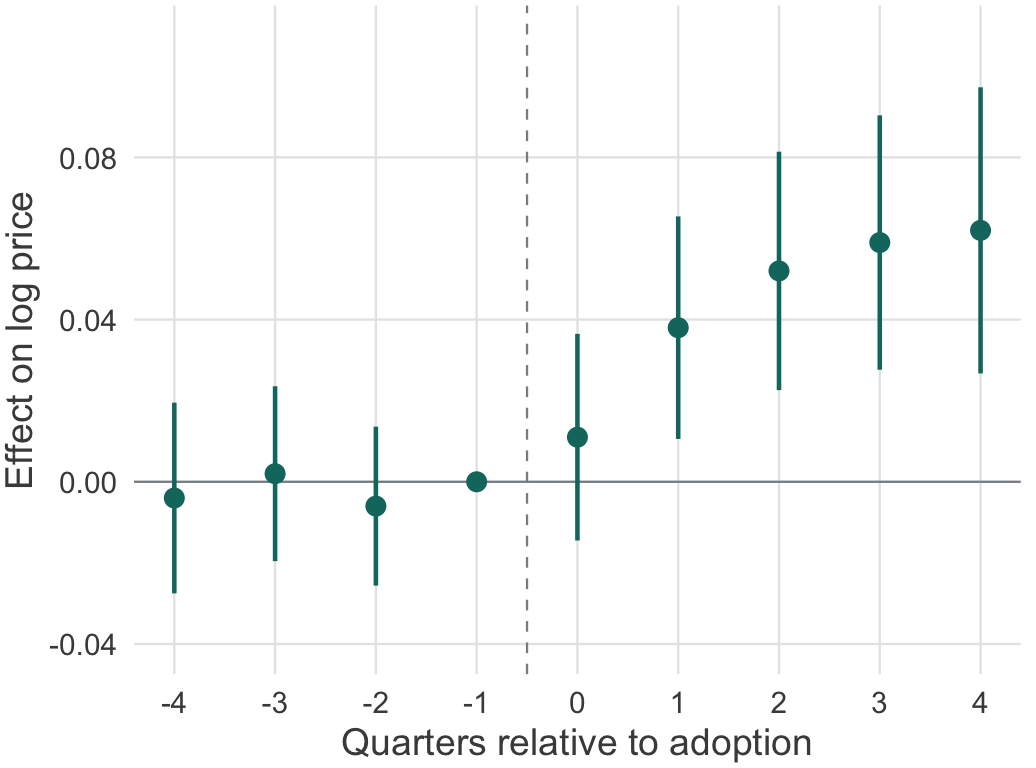
High-exposure markets only. Nothing happens in the four quarters before adoption, the jump lands in the quarter of adoption, and the level persists for a year.
Estimate 0.062 (0.018) four quarters out
Pre-period coefficients are jointly insignificant, \(p = 0.71\).
The interaction survives every specification we can think of
| Outcome: log price | Baseline | Seller trends | Drop 2020 | Balanced | Continuous exposure | Winsorized | PPML |
|---|---|---|---|---|---|---|---|
| Automation × exposure | 0.066 | 0.061 | 0.070 | 0.064 | 0.058 | 0.063 | 0.069 |
| (0.017) | (0.019) | (0.018) | (0.020) | (0.016) | (0.017) | (0.021) | |
| Automation, level | −0.004 | −0.007 | −0.002 | −0.005 | −0.003 | −0.004 | −0.006 |
| (0.011) | (0.012) | (0.011) | (0.013) | (0.010) | (0.011) | (0.014) | |
| Market × week FE | Yes | Yes | Yes | Yes | Yes | Yes | Yes |
| Listings | 41,208 | 41,208 | 38,940 | 22,517 | 41,208 | 41,208 | 41,208 |
Standard errors clustered by market throughout. The continuous-exposure column reports the effect of a one-standard-deviation move in \(\mathrm{RivalShare}_{mt}\). The empirics-first posture, a robust fact ahead of a model, is the one Golder et al. (2023) argue for.
Why the effect is a complementarity
Complementarity follows from the slope of the best response
Proposition 1 Let \(\pi_j(p_j, p_{-j})\) be log-concave in \(p_j\) and suppose automation lowers the adjustment cost \(\kappa_j\). If \(\partial^2 \pi_j / \partial p_j \partial p_{-j} > 0\), then \(p_j^\star = \mathop{\mathrm{arg\,max}}_p \pi_j(p, p_{-j}) - \kappa_j \mathbf{1}\{p \neq p_{j,t-1}\}\) is increasing in \(p_{-j}\), and adoption decisions are strategic complements.
Proof. Log-concavity gives a unique interior maximizer, so \(p_j^\star\) is characterized by the first-order condition. Falling \(\kappa_j\) widens the region where the constraint \(p = p_{j,t-1}\) does not bind, and on that region the cross-partial signs \(\mathrm{d} p_j^\star / \mathrm{d} p_{-j} > 0\) by Topkis. Adopting therefore raises the marginal return to a rival’s adoption.
The empirical interaction is the comparative static the model predicts, not a specification artifact.
Three checks bound the demand-selection threat
Sellers who automate first may be facing rising demand, which would raise prices with or without the API. Three pieces of evidence bound this.
- Adoption timing is uncorrelated with pre-period price and quantity trends once tier is held fixed (\(p = 0.71\) above).
- Within-tier queue position, which is set by a signup date years earlier, gives the same interaction estimate: 0.059 (0.022).
- Rival exposure is not predicted by own-market demand growth, so the interaction is not a demand shock in disguise.
The one case we cannot rule out is a market-level shock hitting exposure and prices together in the same week. We treat this as an open question. Demand dynamics on platforms of this kind are modelled directly by Yin et al. (2024).
What this means for policy
A composition test is what a regulator can actually run
Nothing in the estimate requires a regulator to observe pricing algorithms, which are private, or to prove intent, which is unfalsifiable. It requires the share of a market already automated, which the platform records. Whether firms adopt in the first place is a separate question with its own literature (Dietvorst et al. 2018; Brynjolfsson et al. 2025).
- Below roughly a 40% automated share, permitting automation moves prices by nothing we can distinguish from zero.
- Above it, the same permission is worth 4 to 7 log points, rising in the share.
The threshold is where the fitted interaction crosses zero, so it inherits the standard error on the interaction and should be read as a range.
Automation raises prices where it is already common
Headline estimate 6.2 log points (s.e. 1.4) in the top quartile of rival exposure, −0.4 (1.1) in the bottom quartile, from the same regression.
A rule that permits automated pricing has no single price effect. Its effect is increasing in how much automation the market already has, which makes market composition the object a regulator should be measuring.
Paper and replication files: example.edu/~presenter/repricing
Thank You!
Please contact me with any questions or comments at:
Paper
Appendix
Robustness to the sample window
| Sample or specification | Interaction | s.e. | Level effect | Listings | Markets | Pre-trend \(p\) |
|---|---|---|---|---|---|---|
| Baseline, 2015–2023 | 0.066 | 0.017 | −0.004 | 41,208 | 320 | 0.71 |
| Post-API weeks only, 2019–2023 | 0.071 | 0.021 | −0.002 | 33,415 | 320 | 0.64 |
| Drop the 2020 demand spike | 0.070 | 0.018 | −0.002 | 38,940 | 320 | 0.69 |
| Drop the last adoption cohort | 0.061 | 0.023 | −0.006 | 29,884 | 311 | 0.55 |
| Market-specific linear trends | 0.058 | 0.026 | −0.005 | 41,208 | 320 | 0.83 |
Nothing here moves the estimate by more than half a standard error.
Why we do not instrument adoption with tier eligibility
Tier eligibility is a valid instrument for own adoption and a weak one for the interaction, because the first stage for \(A_{jt} \times \mathrm{RivalShare}_{mt}\) requires exogenous variation in both arguments at once. The available instrument moves only the first.
The reduced form is reported instead: crossing an eligibility threshold raises price by 0.031 (0.012) in high-exposure markets and 0.002 (0.010) elsewhere, a ratio close to the interaction estimate scaled by the 0.48 first stage.
A two-sample approach using a second platform’s queue is in progress.
How automated pricing is measured
The three-distinct-days rule is the middle of three thresholds. Tighter and looser rules move the classified share, but not the estimate.
| Classification rule | Share | Changes per week | Interaction | s.e. | Listings |
|---|---|---|---|---|---|
| Price changes on two or more distinct days | 0.71 | 2.4 | 0.061 | 0.015 | 41,208 |
| Three or more distinct days (baseline) | 0.54 | 3.6 | 0.066 | 0.017 | 41,208 |
| Four or more distinct days | 0.39 | 4.5 | 0.072 | 0.020 | 41,208 |
No listing in the 2015–2018 pre-period crosses the three-day rule for more than two consecutive weeks, which is what makes the threshold usable as a proxy. Imputing the level a listing would have been assigned under an unobserved rule follows Bradlow et al. (2004); richer platform data would allow the transformer approach of Gabel and Ringel (2024) or the multimedia features surveyed in Grewal et al. (2021), and letting a model propose the rule rather than fixing three by hand is the case Ludwig and Mullainathan (2024) make.
References
References
Bradlow, Eric T., Ye Hu, and Teck-Hua Ho. 2004. “A Learning-Based Model for Imputing Missing Levels in Partial Conjoint Profiles.” Journal of Marketing Research 41 (4): 369–81. https://doi.org/10.1509/jmkr.41.4.369.47018.
Brynjolfsson, Erik, Yu (Jeffrey) Hu, and Michael D. Smith. 2003. “Consumer Surplus in the Digital Economy: Estimating the Value of Increased Product Variety at Online Booksellers.” Management Science 49 (11): 1580–96. https://doi.org/10.1287/mnsc.49.11.1580.20580.
Brynjolfsson, Erik, Danielle Li, and Lindsey Raymond. 2025. “Generative AI at Work.” The Quarterly Journal of Economics 140 (2): 889–942. https://doi.org/10.1093/qje/qjae044.
Chevalier, Judith A., and Dina Mayzlin. 2006. “The Effect of Word of Mouth on Sales: Online Book Reviews.” Journal of Marketing Research 43 (3): 345–54. https://doi.org/10.1509/jmkr.43.3.345.
Chevalier, Judith, and Austan Goolsbee. 2003. “Measuring Prices and Price Competition Online: Amazon.com and BarnesandNoble.com.” Quantitative Marketing and Economics 1 (2): 203–22. https://doi.org/10.1023/A:1024634613982.
Dietvorst, Berkeley J., Joseph P. Simmons, and Cade Massey. 2018. “Overcoming Algorithm Aversion: People Will Use Imperfect Algorithms If They Can (Even Slightly) Modify Them.” Management Science 64 (3): 1155–70. https://doi.org/10.1287/mnsc.2016.2643.
Gabel, Sebastian, and Daniel Ringel. 2024. “The Market Basket Transformer: A New Foundation Model for Retail.” Available at SSRN 4335141, ahead of print. https://doi.org/10.2139/ssrn.4335141.
Golder, Peter N., Marnik G. Dekimpe, Jake T. An, Harald J. van Heerde, Darren S. U. Kim, and Joseph W. Alba. 2023. “Learning from Data: An Empirics-First Approach to Relevant Knowledge Generation.” Journal of Marketing 87 (3): 319–36. https://doi.org/10.1177/00222429221129200.
Grewal, Rajdeep, Sachin Gupta, and Rebecca Hamilton. 2021. “Marketing Insights from Multimedia Data: Text, Image, Audio, and Video.” Journal of Marketing Research 58 (6): 1025–33. https://doi.org/10.1177/00222437211054601.
References
He, Sherry, Brett Hollenbeck, and Davide Proserpio. 2022. “The Market for Fake Reviews.” Marketing Science 41 (5): 896–921. https://doi.org/10.1287/mksc.2022.1353.
Ludwig, Jens, and Sendhil Mullainathan. 2024. “Machine Learning as a Tool for Hypothesis Generation.” The Quarterly Journal of Economics, qjad055. https://doi.org/10.1093/qje/qjad055.
Wiles, Emma, Zanele Munyikwa, and John Horton. 2025. “Algorithmic Writing Assistance on Jobseekers’ Resumes Increases Hires.” Management Science, ahead of print. https://doi.org/10.1287/mnsc.2024.04528.
Yin, Mingzhang, Khaled Boughanmi, Anirban Mukherjee, and Asim Ansari. 2024. “Meta-Learning Customer Preference Dynamics for Fast Customization on Digital Platforms.” Available at SSRN 4727171, ahead of print. https://doi.org/10.2139/ssrn.4727171.